Generative AI Is More Than a Model Zoo

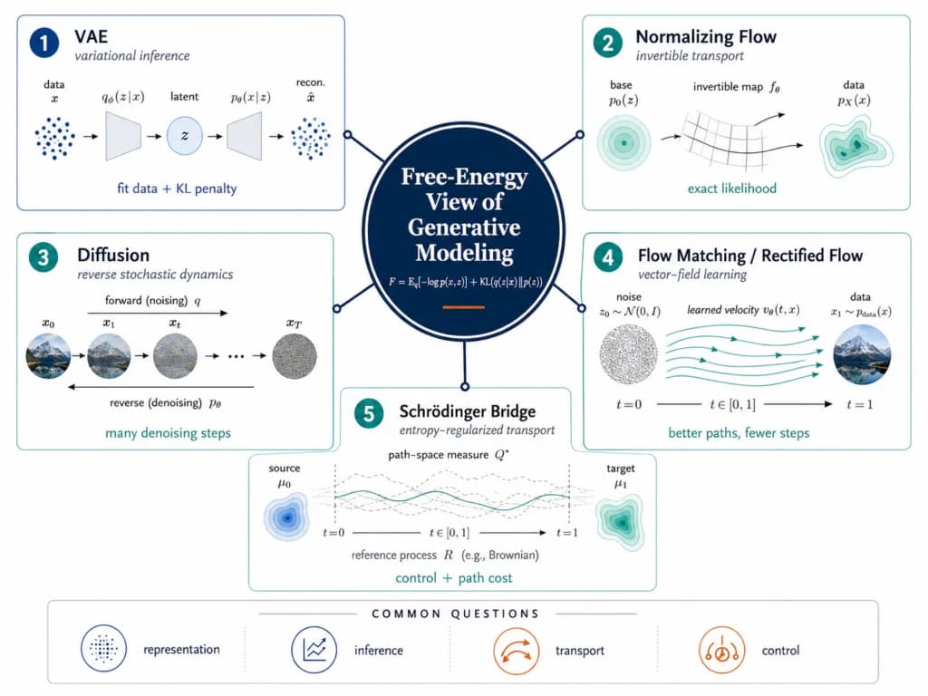
Generative AI is often presented as a parade of model names: VAEs, normalizing flows, diffusion models, flow matching, rectified flow, Schrödinger bridges. That view is useful when you are learning the field for the first time, but it can also make the area look more fragmented than it really is.

A better map is to ask what each family is doing with probability.

Some models approximate inference. Some learn an invertible transport map. Some learn a reverse noising process. Others learn a vector field through probability space, or treat generation as a controlled stochastic path between distributions. The machinery changes, but the underlying questions are the same: how should a model represent uncertainty, how should it move mass, and what price should it pay for complexity?

That is where the language of free energy becomes useful.

In this article, free energy does not need to mean one narrow formula. It is an accounting principle. A model tries to explain the data, but it must also pay for complexity, uncertainty, path cost, or deviation from a prior or reference process. In a VAE, this accounting is explicit in the ELBO. In diffusion models, related accounting appears across many noise levels. In Schrödinger bridges, it appears through entropy-regularized transport on path space.

This is also the lens taken by Max Welling, Sirui Lu, and Lars Holdijk’s forthcoming book Generative AI and Stochastic Thermodynamics: A Tale of Free Energies.^[1] The book is interesting because it does not treat modern generative models as unrelated inventions. It organizes a large part of the field around variational free energy, stochastic dynamics, entropy, transport, and control.

That kind of map is useful because architectures change quickly. The deeper questions last longer.

The free-energy idea in plain language

The phrase “free energy” can sound more mysterious than it needs to.

For the purpose of generative modeling, a useful first definition is this: free energy is a tradeoff between fitting observations and paying for the explanation used to fit them.

A model should explain the data. But explanations are not free. A latent representation can become too complex. A posterior can drift too far from a prior. A path through probability space can be inefficient. A stochastic process can deviate too much from its reference dynamics. Free-energy-style objectives make those costs visible.

The useful way to compare these families is not by asking which one is “best.” It is by asking what each family is paying for. The accounting changes from one model family to another, but the pattern is similar: fit the data, move probability mass, and control the cost of the explanation.

The table is deliberately simplified. It does not make VAEs, flows, diffusion models, flow matching, and Schrödinger bridges identical. It shows why they belong on the same map. Each family has a different mechanism, but each one manages a tradeoff between fit, structure, transport, uncertainty, and cost.

This is not only a philosophical point. It changes how you read model families.

A VAE is not just an encoder and decoder. It is a compromise between reconstruction and regularization. A normalizing flow is not just an invertible neural network. It is a transport map that pays through the change of variables. A diffusion model is not just a denoiser. It learns reverse-time dynamics across a sequence of noisy distributions. Flow matching is not just a faster sampler. It learns a vector field along a probability path. A Schrödinger bridge is not just a fancy diffusion variant. It asks how to move between distributions while staying close to a reference stochastic process.

Once you see the shared accounting problem, the field becomes less noisy.

VAEs: free energy in its most visible form

A variational autoencoder is the easiest place to see the free-energy view because the tradeoff is written directly into the objective.

Kingma and Welling’s VAE paper introduced a scalable stochastic variational inference method for directed probabilistic models with continuous latent variables and intractable posterior distributions.^[2] The key move was to make a variational lower bound trainable with standard stochastic gradient methods using the reparameterization trick.

That sounds formal, but the structure is simple. A VAE learns an encoder, a decoder, a latent variable, an approximate posterior, and a prior. The encoder maps data into a distribution over latent variables. The decoder maps latent samples back into data. The objective rewards good reconstruction while penalizing latent distributions that move too far away from the prior.

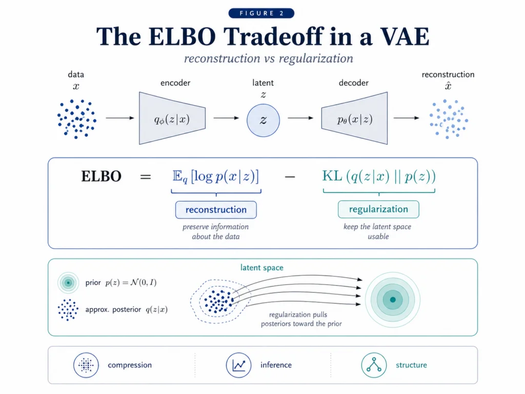
The ELBO, or evidence lower bound, is the training objective behind this tradeoff. In plain language, the ELBO says: preserve enough information to reconstruct the data, but keep the latent space regular enough that sampling still works.

That is why the VAE is more than an old generative model. It is a clean demonstration of the basic accounting problem. If the model is too constrained, reconstructions are weak. If the model is too unconstrained, the latent space becomes less useful. The useful model sits between those extremes.

This is the first free-energy lesson: good generative modeling is not only about fitting the data. It is about fitting the data while controlling the cost of the explanation.

Normalizing flows: transport with exact accounting

Normalizing flows start from a different premise.

Instead of approximating an intractable posterior with a simpler one, a flow transforms a simple density into a more complex density through a sequence of invertible maps. Rezende and Mohamed introduced normalizing flows as a way to construct flexible approximate posterior distributions by applying invertible transformations to an initial density.^[3]

A normalizing flow is a learned transport map. It starts with something easy to sample from, usually a Gaussian, and warps it into something that looks like the data distribution.

The appeal is exact likelihood. Because the maps are invertible, the change-of-variables formula tells you exactly how density changes. When the map stretches or compresses space, the log determinant of the Jacobian accounts for that change.

That is the free-energy intuition here. The model can move probability mass, but the movement is accounted for. The map cannot simply create density for free. It must pay for how it reshapes space.

The cost is architectural. Invertibility and tractable Jacobians constrain what the network can be. This is one reason normalizing flows have not replaced diffusion models for high-fidelity image generation. But flows remain important because exact likelihood is not a minor feature. In density estimation, anomaly scoring, likelihood-ratio problems, and some scientific modeling settings, the ability to evaluate density directly can matter more than visual sample quality.

The lesson from flows is different from the lesson from VAEs. A VAE makes the inference tradeoff visible. A flow makes the transport accounting visible.

Diffusion: generation as learned reverse dynamics

Diffusion models approach the problem by turning generation into a time-indexed process.

The early diffusion paper by Sohl-Dickstein, Weiss, Maheswaranathan, and Ganguli was explicitly inspired by nonequilibrium statistical physics.^[4] The idea was to slowly destroy structure in the data through a forward noising process, then learn a reverse process that restores structure. Ho, Jain, and Abbeel later made denoising diffusion probabilistic models central to modern image generation by training a weighted variational bound connected to denoising.^[5]

The forward process is easy. Add noise to the data until the structure disappears. The reverse process is hard. Learn how to move from noise back toward the data distribution.

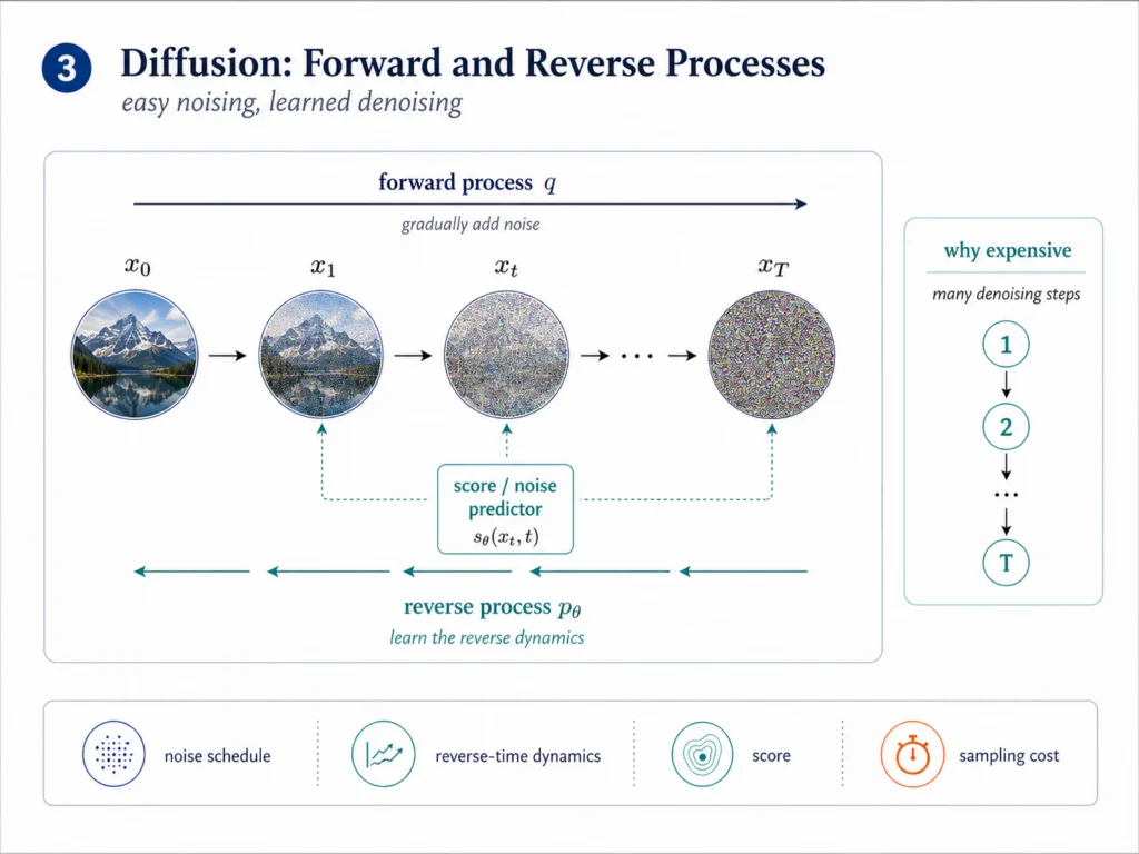
Score-based generative modeling gives this idea a clean continuous-time form. Song and collaborators describe a stochastic differential equation that gradually transforms the data distribution into a known prior, and a reverse-time SDE that transforms the prior back into the data distribution.^[6] The reverse dynamics depend on the score, which is the gradient of the log-density.

A score is a local direction of increasing probability. If the model learns that direction at many noise levels, it can start from noise and move step by step toward structure.

This is where the thermodynamic language starts to feel natural. Diffusion models involve forward and reverse processes, noise schedules, path probabilities, entropy, and the cost of restoring structure. The model is not simply generating an output. It is learning a reverse dynamics.

A careful point matters here. Standard diffusion models are not usually trained as explicit optimal-control problems. It is more accurate to say that they learn reverse-time dynamics, and that the control interpretation becomes sharper when diffusion is viewed through stochastic control, optimal transport, or Schrödinger bridge formulations. That distinction matters because the free-energy view should clarify the field, not overclaim.

Flow matching and rectified flow: making the path explicit

Diffusion models work well, but they often require an iterative path from noise to data. That raises a natural question: can we learn better paths?

Flow matching answers this question by learning a vector field along a probability path. A vector field tells each point where to move and how fast. Lipman and collaborators showed that flow matching can train continuous normalizing flows by regressing vector fields along chosen probability paths, including paths related to diffusion and optimal transport.^[7]

Rectified flow pushes a related idea. Liu, Gong, and Liu proposed learning an ODE that transports between distributions along straighter paths, with the goal of reducing discretization cost and improving sampling efficiency.^[8]

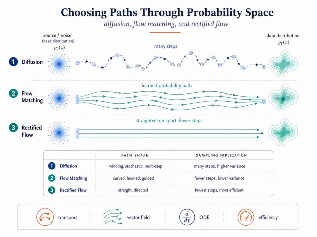
The intuition is geometric. If the path from noise to data is winding and stochastic, sampling may require many steps. If the path is smoother or straighter, fewer numerical steps may be enough. The model family changes because the path has become part of the design.

This is one reason flow matching and rectified flow feel like more than incremental variants. They move attention from endpoint quality to path quality. The question is not only whether the final sample looks right. The question is how efficiently and stably the model gets there.

In a free-energy view, that is exactly the kind of question we should expect. The model is still fitting data, but it is also paying for the route it takes through probability space.

Schrödinger bridges: when the path itself is the object

Schrödinger bridges are the most abstract part of this map, so they deserve a plain definition.

A Schrödinger bridge asks how to move one probability distribution into another through stochastic trajectories while staying close to a reference process, often Brownian motion. It is an entropy-regularized optimal transport problem on path space.

Unpack that sentence piece by piece.

Optimal transport asks how to move probability mass from one distribution to another. Entropy regularization keeps the solution from becoming too rigid. Path space means we care about full trajectories, not only starting and ending points. A reference process gives the system a baseline dynamics that it can deviate from, but not without paying a cost.

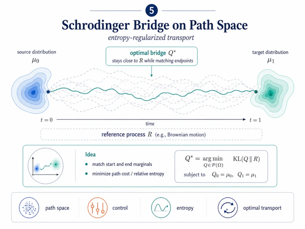
De Bortoli, Thornton, Heng, and Doucet connected Schrödinger bridges to score-based generative modeling, framing diffusion Schrödinger bridges as a way to build finite-time diffusion processes for generative modeling.^[9]

This is where the free-energy framing becomes more than a metaphor. Generation is not only about the endpoint distribution. It can also be about the path.

This is conceptually similar to type theory, where different proofs of the same statement need not be treated as identical. The theorem is the endpoint, but the proof still carries structure. Likewise, two generative models may target the same distribution while taking different paths through probability space. Those paths matter because they encode efficiency, stability, inductive bias, and control. In that sense, a generative model is not just a distribution. It is a program for producing one.

That matters in domains where trajectories have meaning. In robotics, the path of an action matters, not just the final pose. In scientific simulation, the evolution of a system matters, not just the final state. In inverse problems, the route from prior uncertainty to posterior structure can encode constraints, uncertainty, and cost.

Schrödinger bridges are not the simplest production tool. They are mathematically heavier than VAEs, normalizing flows, and many diffusion pipelines. But they are conceptually important because they show where the field is going: from generating samples toward controlling stochastic processes.

What this map explains, and what it does not

The free-energy view gives structure to a field that can otherwise look like a stream of unrelated paper titles. It explains why VAEs, flows, diffusion models, flow matching, and Schrödinger bridges keep touching the same ideas: inference, transport, entropy, uncertainty, cost, and control.

But the framing has limits. It is useful because it connects the training and transport side of generative modeling. It is not a substitute for evaluation, calibration, safety, or domain-specific validation.

The free-energy view tells us more about training and generation than evaluation. It helps explain how models learn distributions and move through probability space. It does not, by itself, tell us whether a generated molecule is synthesizable, whether a forecast is calibrated, whether a robot action is safe, or whether a generated proof is correct.

As generative models move deeper into science, engineering, robotics, forecasting, and software systems, sample quality is no longer enough. We need models that can be controlled, evaluated, constrained, and integrated into real workflows.

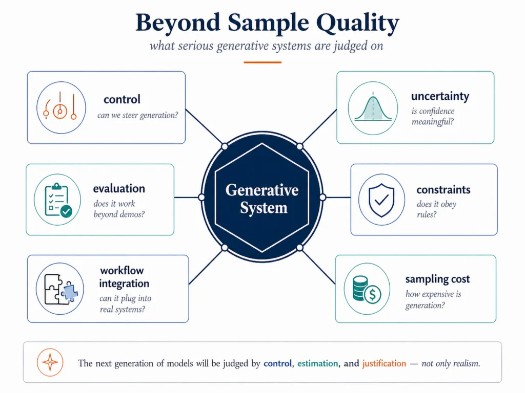
This is why the free-energy lens is useful but not final. It gives a serious language for inference, uncertainty, path cost, and control. It does not eliminate the need for domain-specific evaluation.

Conclusion

Generative AI is easier to understand when we stop treating model families as isolated inventions.

VAEs show the tradeoff between reconstruction and regularization. Normalizing flows show how exact likelihood can be preserved through invertible transport. Diffusion models show how generation can be framed as learned reverse dynamics. Flow matching and rectified flow make the probability path itself more explicit. Schrödinger bridges show how generation can become controlled stochastic transport on path space.

The details differ, but the accounting problem keeps returning. Fit the data, but pay for the explanation. Move probability mass, but pay for the transport. Reverse noise, but pay for the path. Control a stochastic process, but pay for deviating from the reference dynamics.

That is why the free-energy view is valuable. It is not the whole answer, and it does not explain every generative model. But it gives a durable map of a field that often looks more chaotic than it is.

The next generation of generative systems will not be judged only by how realistic their samples look. They will be judged by whether they can control the generation process, quantify uncertainty, obey constraints, reduce cost, and justify their outputs in settings where mistakes matter.

Free energy is a serious candidate for a unified and precise language that connects inference, uncertainty, transport, and control.

References

- [1] Max Welling, Sirui Lu, and Lars Holdijk. Generative AI and Stochastic Thermodynamics: A Tale of Free Energies. Cambridge University Press, forthcoming 2026. cambridge.org
- [2] Diederik P. Kingma and Max Welling. “Auto-Encoding Variational Bayes.” 2013. arXiv:1312.6114
- [3] Danilo J. Rezende and Shakir Mohamed. “Variational Inference with Normalizing Flows.” ICML/PMLR, 2015. proceedings.mlr.press
- [4] Jascha Sohl-Dickstein, Eric A. Weiss, Niru Maheswaranathan, and Surya Ganguli. “Deep Unsupervised Learning using Nonequilibrium Thermodynamics.” 2015. arXiv:1503.03585
- [5] Jonathan Ho, Ajay Jain, and Pieter Abbeel. “Denoising Diffusion Probabilistic Models.” 2020. arXiv:2006.11239
- [6] Yang Song, Jascha Sohl-Dickstein, Diederik P. Kingma, Abhishek Kumar, Stefano Ermon, and Ben Poole. “Score-Based Generative Modeling through Stochastic Differential Equations.” 2020. arXiv:2011.13456
- [7] Yaron Lipman, Ricky T. Q. Chen, Heli Ben-Hamu, Maximilian Nickel, and Matt Le. “Flow Matching for Generative Modeling.” 2022. arXiv:2210.02747
- [8] Xingchao Liu, Chengyue Gong, and Qiang Liu. “Flow Straight and Fast: Learning to Generate and Transfer Data with Rectified Flow.” 2022. arXiv:2209.03003
- [9] Valentin De Bortoli, James Thornton, Jeremy Heng, and Arnaud Doucet. “Diffusion Schrödinger Bridge with Applications to Score-Based Generative Modeling.” NeurIPS 2021. openreview.net
- [10] Laurent Dinh, Jascha Sohl-Dickstein, and Samy Bengio. “Density Estimation using Real NVP.” ICLR 2017. arXiv:1605.08803